
|
Yet Another Comparison Between a
Better Light Scanning Back and Several Popular DSLRs... |
||
|
...without bothering with the DSLRs!
|
||
|
An explanation and demonstration of the fundamental differences between interpolated color
(Bayer pattern) digital camera images and full-color scanning back images |
||
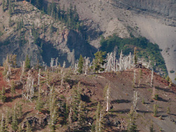
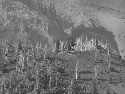
by Mike Collette, founder of Better Light, Inc. Perhaps the most familiar photographic equipment comparison involves seeing how well different systems can reproduce fine detail. While the color accuracy and dynamic range of a photographic image are somewhat independent of format, the ability to record fine detail is generally directly related to the size of the image capture device, and is one of the reasons why some photographers use larger cameras. When doing these “resolution” comparison tests, any disparity in image size or focus caused by magnification or perspective inconsistencies among cameras, as well as any discrepancy in image brightness or contrast caused by variations in exposure, will make the results harder to compare accurately. When multiple systems are involved, the skill and care with which the cameras are set up, as well as how the capture devices are operated, might also skew the results in favor of a more familiar or easier-to-use system. To more accurately demonstrate the differences in sharpness and resolution between an uninterpolated image from a Better Light scanning back and interpolated images from several current DSLR cameras utilizing Bayer pattern sensors, this article will use straightforward simulation techniques to derive the (lower-resolution) DSLR images directly from the (higher-resolution) Better Light image data. In this manner, the image composition, focus, and exposure are perfectly consistent among all examples, and the primary variance will be from differences in the number of pixels in each image. While some readers will immediately be suspicious because I’m not using actual DSLRs for this comparison, I hasten to remind them that, besides having more pixels, many other attributes of a Better Light system are also superior to the DSLRs, so if anything these simulated results might be better than what one could obtain from the actual hardware. Besides, my objective isn’t so much to compare specific hardware devices as to compare different capture methods, as exemplified by currently-available devices. Let’s cut to the chase and show the results from this comparison first, and then interested and/or disbelieving readers can continue on to see how these results were obtained. Since many large-format lenses work best at infinity focus, I started with a landscape photo of Crater Lake that I captured last year using my very sharp Rodenstock 135mm Apo-Sironar S lens with a Better Light model 6000-HS scanning back: |
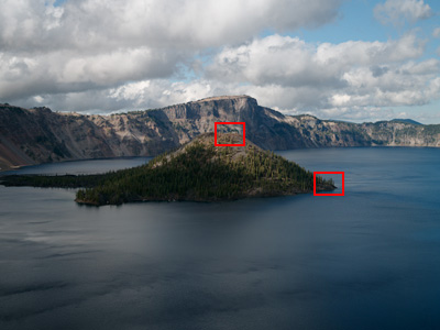 |
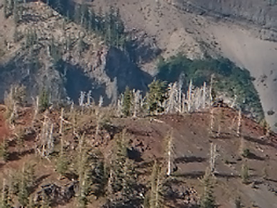
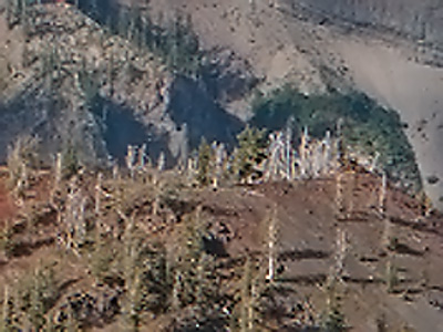
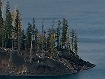
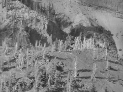
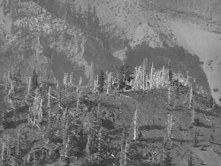
From the entire image (left), two 300 x 400 pixel sections were copied and saved as examples of the 144 megapixel scanning back image. These example sections were selected to contain both high and low contrast highlight and shadow detail, along with a selection of natural colors. Copies of these two sections were then processed as described below to yield images equivalent to a 39 megapixel DSLR image, and a 16 megapixel DSLR image. Finally, the simulated DSLR images were interpolated up to match the size of the original scanning back sections to more clearly demonstrate the differences, and moderate sharpening was applied to all of the comparison images. before saving them as high-quality JPEGs for this article. |
|||
|
|
||||
 |
 |
|||
|
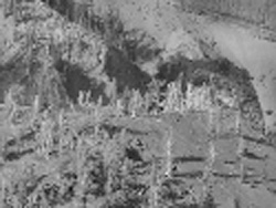
144 megapixel scanning back
|
||||
 |
 |
|||
|
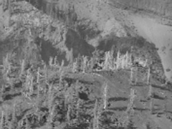
39 megapixel DSLR simulation, interpolated
|
||||
 |
 |
|||
|
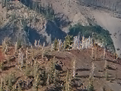
16 megapixel DSLR simulation, interpolated
|
||||
|
CLICK HERE to download one megabyte layered TIFF file
containing all three images of the example above. |
CLICK HERE to download one megabyte layered TIFF file
containing all three images of the example above. |
|||
|
You can download one megabyte layered TIFF files containing all three images of each section. By turning on/off the visibility of each layer of the TIFF files, one can quickly switch among the 144, 39, and 16 megapixel images for a much clearer view of the differences. |
||||
|
These results might look a little different than comparisons made using a still-life subject, in part because this large format landscape photo contains considerably more fine detail than a close-up photo of a camera or doll. Furthermore, there isn’t any difference in size, brightness, contrast, or color among these images, other than those changes introduced by the pixel processing, so it’s easier to see more subtle differences. Finally, these images are shown at their pixel sizes described in this article, without any subsequent “resizing for publication”, as has sometimes occurred in other comparisons. Since the beginning of silver-based photography, using a larger camera has generally allowed the photographer to make a larger, higher-quality printed reproduction. Digital cameras have complicated this issue somewhat by introducing a wider variety of pixel sizes and capture technologies than was previously available, often providing better performance than an equivalent film format. With digital imaging, the amount of information being captured is not always just a function of the size of the capture device. However, it is still safe to say that recording a greater amount of original information for each image will allow the photographer to make a larger, higher-quality printed reproduction. Because of the almost universal use of Bayer pattern image sensors in instant-capture digital cameras, many readers might think that the megapixel rating of a digital camera is only an expression of its pixel dimensions, since this happens to be true for the vast majority of digital cameras on the market. However, the (former) JCIA megapixel rating specification is really intended to express the information-capturing ability of a digital camera, so three-CCD and scanning cameras are allowed to count all three colors of their pixels, even though the different-colored pixels are effectively stacked on top of each other. The additional full-color pixel data from the scanning back represents considerably more image information than is captured by a Bayer pattern sensor – hence, the considerably higher megapixel rating for the scanning back. As has also been true since the beginning of photography, not all photographers will need or want to use a larger camera, let alone a digital scanning back. Using a large format camera is a much slower and more deliberate process than using a DSLR, imposing some constraints on suitable subjects and shooting conditions, and using a scanning back further limits these choices. However, when conditions allow, the greater information recording capability of the scanning back, combined with today’s wide-format photographic printing technologies, gives photographers unprecedented ability to create very large prints with outstanding detail and clarity, even upon close inspection. Of course, not all photographic subjects will benefit from such large reproductions, but I suspect that I’m not the only landscape photographer who likes to see my large-scale scenic images printed as large as possible.Details of the simulation process: Simulating an instant-capture digital image from the commonly-used Bayer pattern sensor involves more than simply reducing the pixel dimensions of the larger scanning back image to those of the DSLR image. This is because the scanning back image contains actual red, green, and blue pixel data at every spatial location in the image, whereas two-thirds of the DSLR image has been interpolated from a single matrix of red, green, and blue pixels, typically arranged as shown in the illustration below. |
||||||||||||
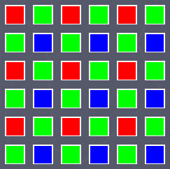 |
Because each color is only sensed by some of the pixels in the Bayer matrix, each color channel will collect only a portion of the information that is recorded by the full-color scanning back. For example, the simple 6 by 6 matrix of pixels shown contains:
|
|||||||||||
|
Bayer RGB Pixel Pattern
|
||||||||||||
There is also an apparent offset among the color channels caused by the physical offset among the pixels. For example, if the array shown above was uniformly illuminated, the red channel response would be diagonally displaced from the blue channel response, with the green channel somewhere in between. You can see this by looking at the relative positions of the red and blue pixels in the above array. After image capture, each color channel of image data from a Bayer pattern sensor is usually enlarged to the full size of the array, with the missing pixels in each color channel interpolated from nearby pixels of the same color. Aggravated by the offsets among the color channels, this interpolation often causes colored artifacts to appear in areas of high-contrast fine detail, commonly known as “color aliasing” artifacts. Image processing is used to avoid or remove these artifacts, sometimes by putting a slight blurring filter in front of the sensor (an “anti-aliasing filter”), and often by post-processing the image data using sophisticated color noise removal algorithms. This demonstration uses several different image resizing methods available in Photoshop to derive the DSLR images, each where it is most appropriate: 1. “Nearest Neighbor” interpolation – a simple method of resizing an image that first determines from where in the existing pixel array each new pixel must be derived, and then picks the nearest single pixel from the existing array to represent the value of the new pixel. Really not “interpolation” because no new or intermediate values are generated -- just copies of the existing values. 2. “Bilinear” interpolation – a somewhat more complicated method of resizing an image that first determines from where in the existing pixel array each new pixel must be derived, and then calculates a new value from the values of the existing pixels around each new pixel, using linear proportioning. Generates a smooth result using all of the original image information. 3. “Bicubic” interpolation – an even more complicated method of resizing an image that first determines from where in the existing pixel array each new pixel must be derived, and then calculates a new value from the values of the existing pixels around each new pixel, using nonlinear polynomial proportioning. Can generate a sharper-looking result than Bilinear interpolation, but may not be as faithful to the original image information. The process for simulating lower-resolution Bayer pattern image data involves the following steps, shown here with image examples for the 16 megapixel DSLR simulation. 1. Make a copy of the 144 megapixel example section, and reduce the pixel dimensions of this section using Bilinear interpolation to be equal to the pixel dimensions of an equivalent section from a 16 megapixel DSLR. (See below for the pixel dimension calculations.) This reduced-resolution section from the scanning back still has three times as much information as a Bayer pattern DSLR image. |
||||||||||||
 |
 |
||||
|
Original 144 Megapixel Section
|
Initial Reduction
|
||||
|
2. Make a copy of each individual color channel as a new (grayscale) image, and reduce the pixel dimensions of each color channel independently to be equal to the number of pixels in each color channel of an equivalent section from a 16 megapixel DSLR. (See below for the pixel dimension calculations.) Use Nearest Neighbor interpolation for the red and blue channels, and Bilinear interpolation for the green channel. To simulate the offset among color channels, rotate the blue channel 180 degrees before reducing its pixel dimensions -- because each image section contains an even number of pixels in each dimension, and each section is being reduced by exactly one-half in each dimension, Nearest Neighbor interpolation will choose different pixels for the rotated blue channel than for the un-rotated red channel. Rotate the blue channel another 180 degrees after this reduction to restore its proper orientation. Bilinear interpolation is used for the green channel to provide more uniformly distributed results than Nearest Neighbor interpolation would yield. |
|||||
 |
 |
|||
|
Red Channel
|
|
Resampled Red
|
||
 |
 |
|||
|
Green Channel
|
|
Resampled Green
|
||
 |
 |
|||
|
Blue Channel
|
|
Resampled Blue
|
||
|
|
3. The reduced grayscale images of the three color channels now represent the actual image data captured by a Bayer pattern sensor. The green channel image is larger than the other two because there are more green pixels on the sensor. Each color channel image is now interpolated to its final pixel dimensions using Bicubic interpolation - less of an increase is needed for the green channel than for the other two channels to produce three equal-sized image planes. |
|
 |
|||
| Resampled Red |
Interpolated Red
|
|||
|
 |
|||
| Resampled Green |
Interpolated Green
|
|||
|
 |
|||
| Resampled Blue |
Interpolated Blue
|
 |
|
|||
|
|
Recombined Color Image
|
|||
 |
|
|||
|
Filtered Color Image
|
||||
|
|
||||
 |
|
|||||
|
Sharpened Color Image
|
Interpolated and Re-Sharpened Final Image
|
|
Calculations used for the simulation process: |
||||
| Pixel dimensions of a 144 megapixel scanning back | 6000 by 8000 pixels | |||
| Pixel dimensions of a 39 megapixel digital back | 5412 by 7216 pixels | |||
| Pixel dimensions of a 16 megapixel digital SLR | 3328 by 4992 pixels | |||
| Ratio of 39 MP to 144 MP pixel dimensions | 0.902 by 0.902 | |||
| Ratio of 16 MP to 144 MP pixel dimensions | 0.555 by 0.624 | |||
| Ratios used for the initial pixel reduction | 0.905 for the 39MP simulation | |||
| (to produce even numbers for the reduced pixel dimensions) | 0.625 for the 16MP simulation | |||
| (0.625 for 16 MP uses full width of sensor, assumes some vertical cropping) | ||||
| Pixel dimensions of each 144 MP example section | 300 by 400 pixels | |||
| Total sensor pixels in each 144 MP section | 300 x 400 x 3 = 360,000 pixels | |||
| Total RED pixels in each 144 MP section | 300 x 400 = 120,000 pixels | |||
| Total GREEN pixels in each 144 MP section | 300 x 400 = 120,000 pixels | |||
| Total BLUE pixels in each 144 MP section | 300 x 400 = 120,000 pixels | |||
| Pixel dimensions of each 39 MP example section | 272 by 362 pixels | |||
| Total sensor pixels in each 39 MP section | 272 x 362 = 98,464 pixels | |||
| Total RED pixels in each 39 MP section | 136 x 181 = 24,616 pixels | |||
| Total GREEN pixels in each 39 MP section | 192 x 256 = 49,152 pixels | |||
| Total BLUE pixels in each 39 MP section | 136 x 181 = 24,616 pixels | |||
| Pixel dimensions of each 16 MP example section | 188 by 250 pixels | |||
| Total sensor pixels in each 16 MP section | 188 x 250 = 47,000 pixels | |||
| Total RED pixels in each 16 MP section | 94 x 125 = 11,750 pixels | |||
| Total GREEN pixels in each 16 MP section | 133 x 177 = 23,541 pixels | |||
| Total BLUE pixels in each 16 MP section | 94 x 125 = 11,750 pixels | |||
| Ratio of 39 MP to 144 MP total sensor pixels | 27 percent | |||
| Ratio of 16 MP to 144 MP total sensor pixels | 13 percent* | |||
| (* for this example - 16 MP is higher than expected due to using full width of sensor) | ||||